Activation Patching Explained: Finding Causes Inside a Model

You can watch a language model give the right answer and still have no idea which parts of it did the work. This post gives you activation patching explained: swap one internal activation between two runs and see what changes. By the end you will know how to set up a clean run and a corrupted run, which number to measure, and where the method can mislead you.

Activation patching explained in plain words

Activation patching is an experiment on a neural network. You take an internal value from one forward pass and paste it into another, then check whether the output moves. Zhang and Nanda's 2023 paper on best practices calls it a standard technique for finding the important parts of a model, also known as causal tracing or interchange intervention.

Think of two nearly identical prompts: one leads the model to answer A, the other to answer B. If copying one part's activation from the first run into the second flips the answer back toward A, that part carries information the model uses to choose A. Everything else is detail about which activations to swap and how to score the result.

Why reading activations is not enough

Many interpretability methods only observe. The logit lens decodes each layer to show a prediction forming, and a linear probe shows what information can be read out. Both show what is present, not what the model uses.

Patching intervenes. You change one thing and hold the rest fixed. If the output changes, you have evidence of a causal role, not just a correlation: the logic of a controlled experiment, applied to a network's insides.

How it works: clean, corrupted and patched runs

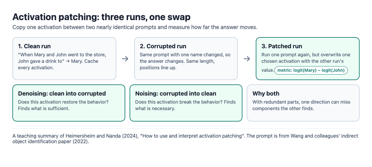
Three runs and one swap, with the two directions you can patch in.

1. Clean run. Run the model on a prompt where it shows the behavior you care about, and save the activations.
2. Corrupted run. Run it on a minimally different prompt where the behavior changes. Keep the length and structure the same so positions line up.
3. Patched run. Run one prompt again, but at one chosen place (a layer, a token position, an attention head or an MLP output) overwrite the activation with the value from the other run.

Repeat the patched run for each place you want to test, and you get a map of where the behavior lives.

Heimersheim and Nanda's 2024 guide, "How to use and interpret activation patching", names two directions. Denoising patches clean activations into the corrupted run and asks which ones are sufficient to restore the behavior. Noising patches corrupted activations into the clean run and asks which ones are necessary, because swapping them breaks it. The guide stresses that the two are not mirror images, and knowing which one you ran matters when you read the map.

Measuring the effect: logit difference

You need one number per patch. Heimersheim and Nanda recommend the logit difference: the logit of the correct answer minus the logit of the competing one. Where metrics disagree, they write that they trust logit difference most, partly because it is easy to attribute directly to individual parts of the model.

To compare patches, you can scale each result between the two runs: 1 means the patch fully restored the clean result, 0 means it did nothing. Two habits keep you honest. Check that the clean and corrupted runs really differ by a clear margin, and average over many prompt pairs rather than trusting one.

A worked example: the indirect object task

Wang and colleagues' 2022 paper "Interpretability in the Wild" studied how GPT-2 small completes sentences like this one:

• Clean: When Mary and John went to the store, John gave a drink to. The answer should be Mary.
• Corrupted: the same sentence with one name changed, so the expected answer changes.

Your metric is logit(Mary) - logit(John). Here is how a study like this proceeds, step by step:

1. Patch the residual stream at every layer and position, and see where restoring the clean value restores the answer.
2. Narrow down to attention heads at the final position. Look at what high-scoring heads attend to.
3. Use path patching, the paper's own method, to change one route between heads while freezing others, so you can test claims about connections, not just parts.
4. Check the result over many prompt pairs with different names and templates.

The paper's explanation covers 26 attention heads in 7 main classes. In its account, Duplicate Token Heads notice the repeated name, S-Inhibition Heads stop the later heads from attending to it, and Name Mover Heads copy the remaining name, Mary, to the output.

Causal tracing for facts

Meng and colleagues' 2022 ROME paper used a version called causal tracing to find where a model recalls facts. Instead of a second prompt, they added noise to the embeddings of the subject's tokens, then restored clean states one at a time. Their results pointed to middle-layer feed-forward modules at the last subject token.

Pitfalls: backup heads, redundancy and odd inputs

• Backup heads. In the indirect object circuit, Backup Name Mover Heads do not normally move the name, but take over when the main Name Mover Heads are knocked out. Remove one part and the network may compensate, so the part can look less important than it is.
• Redundancy. Heimersheim and Nanda show that when two parts are both needed, noising finds both and denoising can miss them; when either one is enough, the reverse happens. That is why it helps to run both directions.
• Inputs the model never sees. Replacing an activation with zeros or a dataset average can push the model into states it never meets in training. The guide recommends patching from a matched corrupted prompt, which tends to keep the model closer to normal.
• Choices change answers. Zhang and Nanda found that changing the metric or the way you corrupt the prompt can lead to different interpretability results. Your corrupted prompt defines the question you are asking.

None of this makes the method useless. Each result is a claim to test further, not a final answer.

Frequently asked questions

How is activation patching different from the logit lens?

The logit lens reads intermediate layers to see what the model predicts so far, which is observation. Activation patching changes an activation and measures the effect, which gives causal evidence about what the model uses.

Is activation patching the same as activation steering?

No. Patching swaps in activations from another real run to find where a behavior is computed. Activation steering adds a chosen direction to change behavior on purpose.

What is the difference between noising and denoising?

Denoising patches clean activations into a corrupted run to find what is sufficient for the behavior. Noising patches corrupted activations into a clean run to find what is necessary.

Is there a faster version?

Yes. Heimersheim and Nanda mention attribution patching as a fast approximation; you then confirm the most promising parts with real patches.

Get started

Activation patching is one tool within interpretability. On Learn AI Alignment Theory, Interpretability is one of 7 Advanced courses, next to Scalable Oversight, The Science of LLM Misalignment and Agent Foundations. If you are newer, the 5 Basic courses, starting with What Is Alignment? and How Modern AI Works, need no background. For more on this group, read induction heads explained.

Each lesson takes about 8 minutes, lists its sources and separates what is known from what is still open. Debate cards set out each serious position with no verdict, and a 349-term glossary helps with the vocabulary. You sign in with Google or an emailed code.

Start Learn AI Alignment Theory: short hands-on lessons from first principles to open research, with every side of every debate and the sources to read next.