Attribution Patching Explained: A Faster Way to Find Circuits

Attribution patching explained: a faster way to find circuits means a shortcut for one of interpretability's most expensive jobs, working out which parts of a neural network cause a given behavior. It estimates the answer with gradients, using two forward passes and one backward pass, in place of one run for every component. This post follows the two papers that matter most: the 2023 edge attribution patching paper and the 2024 AtP* paper.

If you want to study interpretability in short lessons, Learn AI Alignment Theory has an Advanced Interpretability course and a glossary of 349 terms, and it sets out where researchers disagree, without picking a side.

Attribution patching explained: a faster way to find circuits

The goal of mechanistic interpretability is to find the parts of a model, called a circuit, that are responsible for a specific task. To know whether a part matters, researchers use activation patching: take the activation of one component from a different run, put it into the run you care about, and see how much the output metric changes.

Attribution patching estimates that change without doing the patch. The AtP* paper credits the method to Nanda (2022) and describes it as a fast, gradient-based approximation to activation patching.

The problem: one patch needs one forward pass

Activation patching is exact for the patch it makes, but each patch costs a forward pass. The AtP* authors note that a sweep over every component scales linearly with the number of components, so the number of forward passes can climb into the millions or billions.

Their own example: on a prompt of length 1024, Chinchilla 70B has 2.7 billion neuron nodes. Patching each one separately would take about 2.7 billion forward passes for a single prompt pair, before averaging over many prompt pairs. That is the cost attribution patching removes.

How attribution patching works

The idea is calculus. You have a metric L, such as the loss or the gap between the correct and wrong answer. You want to know how L would change if you swapped one activation from the clean run for the one from a corrupted run. Syed, Rager and Conmy write this as a first-order Taylor expansion: the change is approximately the difference between the two activations times the gradient of L with respect to that activation.

1. Run the clean prompt forward and save the activations.
2. Run the corrupted prompt forward and save its activations.
3. Run one backward pass on the clean run. The gradients you need are intermediate terms of an ordinary backward pass.
4. Multiply and read off the scores. Each component gets an estimate of how much patching it would change the metric.

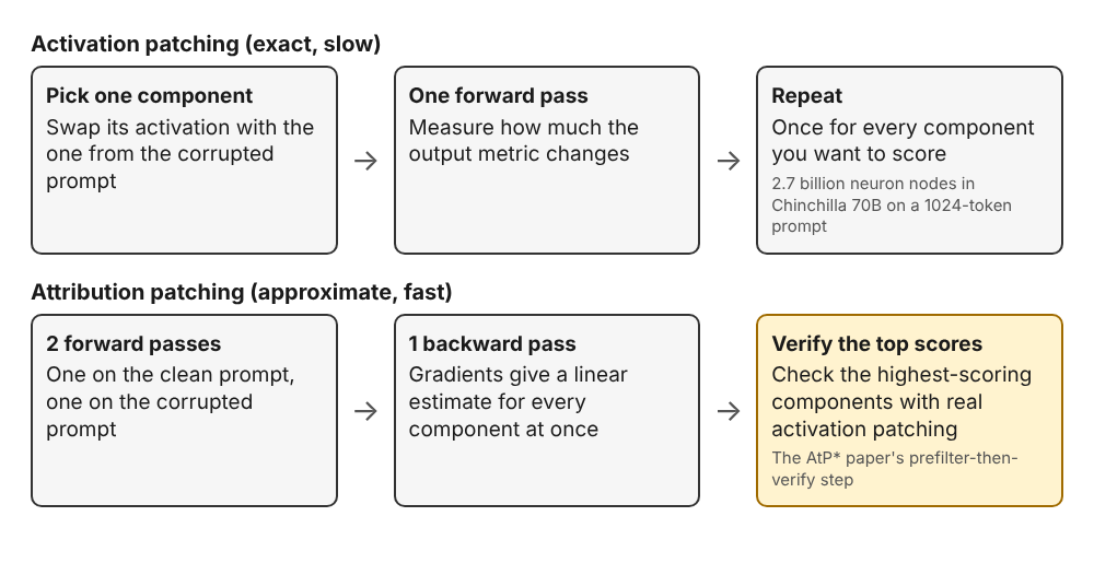
That is two forward passes and a backward pass for every component at once, where activation patching needs a separate pass per component.

A worked example with the papers' own numbers

Take the AtP* authors' figure of 2.7 billion neuron nodes for one 1024-token prompt. This is the session's own arithmetic on their number, not a result from the paper:

• Exact patching of every neuron: about 2.7 billion forward passes.
• Attribution patching: 2 forward passes and 1 backward pass for the same scores.
• Then verify: the paper's recommended use is as a prefilter. Sort nodes by the size of the estimate and check the top ones with real activation patching. The authors note that researchers usually care about a small set of top contributing nodes, so verification costs far less than a full sweep.

The estimate is a cheap ranking. The patch is the confirmation.

From scores to circuits: edge attribution patching

Syed, Rager and Conmy turn the idea into a circuit-finding method. They treat a language model as a graph and score every edge, meaning an activation passed between two components. They keep the top k edges as the circuit. They call this Edge Attribution Patching, and they compare it with automated circuit discovery (ACDC) on three tasks where earlier studies had found circuits to use as ground truth: indirect object identification, docstring completion, and greater-than.

The scores they report are AUC values, where 1.0 means the method recovers the known circuit perfectly:

• Indirect object identification: 0.904 for their method, against 0.588 for ACDC with the task metric and 0.868 with KL divergence.
• Greater-than: 0.896, against 0.458 and 0.849.
• Docstring: 0.976, against 0.972 and 0.982. Here ACDC with KL divergence scored higher, and exact activation patching scored 0.978.

Averaged over all tasks, their method has the greater AUC, which is the paper's headline claim. It is a claim about small models on three known circuits, so read it that way. For what circuits mean in practice, see circuits in neural networks.

Where the approximation fails

The same paper tests how faithful the shortcut is, and the answer is mixed. On the docstring task, attribution patching scores and activation patching scores correlated only weakly (R squared of 0.27). The best-fit line had a gradient of 0.531, which the authors read as attribution patching estimating the effect as twice as important as it really is. They also note that the method does not work if the gradient of the metric is zero, which is why they avoid KL divergence there.

The AtP* paper explains a deeper reason, and finds two classes of failure that cause false negatives, meaning real causes the shortcut misses:

• Attention saturation. If the clean run sits in a flat region of the softmax, the local gradient says little about what happens when the activation changes a lot.
• Cancellation. A component can have a direct effect and an indirect effect that nearly cancel. A small error in the linear approximation can then make the estimate orders of magnitude too small.

Their fixes are two changes. When patching queries and keys, recompute the attention softmax instead of relying on the gradient there. And use dropout on the backward pass (GradDrop) so that cancelling effects are less likely to hide each other. They also give a diagnostic that bounds the probability of false negatives that remain.

What this means for alignment research

Syed, Rager and Conmy say that scaling interpretability to large models could address concerns about transparency, as well as speculative risks about the alignment of machine learning systems. Nothing in the two papers shows that has happened yet. Both study how to find circuits cheaply, not whether the circuits explain risky behavior.

Cheaper localization still matters because it widens what researchers can look at. A different line of work traces whole computations through a model, as in circuit tracing in language models. Whether that scales to the models people worry about is an open question, and researchers differ on how much interpretability will help. The app's 71 debate cards state each serious position fairly with no verdict.

Frequently asked questions

What is the difference between activation patching and attribution patching?

Activation patching swaps in an activation and measures the real change in the output. Attribution patching estimates that change from gradients, so it needs only two forward passes and one backward pass for many components.

Is attribution patching exact?

No. It is a linear approximation. The edge attribution patching paper found a weak correlation with activation patching on one task, and the AtP* paper names two failure modes that cause false negatives.

What is AtP*?

It is a variant from Google DeepMind researchers that fixes the two failure modes by recomputing the attention softmax for queries and keys and by using dropout on the backward pass. It comes with a way to bound remaining false negatives.

Do I need to know calculus to follow it?

Only the idea of a gradient: it tells you how much a number changes when you nudge an input. The papers use it to guess what a patch would do before doing it.

Get started with Learn AI Alignment Theory

Lessons take about 8 minutes each and include questions and hands-on activities. You sign in with Google or an emailed code, and you need to be 13 or older. You can read more on the about page.

Start Learn AI Alignment Theory: short hands-on lessons from first principles to open research, with every side of every debate and the sources to read next.